4.The effect of the stellar passage on the cometary perihelion
distance.
This is an abbreviated and translated version of Chapter 4 of my
PhD
thesis: "Stellar perturbations on the Oort cloud", prepared in 1990
under supervision of prof. Hieronim Hurnik.
This page was created 1 Feb.
2006 and last modified 2 Feb. 2006. This page is still under
construction, I will add more text later. All figures are "clickable",
allowing postscript versions to be downloaded.
Our main field of interest is the gravitational influence of the
passing star on the perihelion distance of a comet in the Oort cloud.
We are specially interested in such cases when the perihelion distance
is decreased below the observational limit, assumed to be 10 AU. We
present here only the effects of the singular stellar passage through
or near the Oort cloud.
Below, in several examples, we show how the change in cometary
perihelion distance depends on the parameters and geometry of the
stellar path. W start with planar cases, when a star moves in the comet
orbital plane.
4.1. Planar cases
We have two different cases here: when the star moves outside the
cometary orbit and when it crosses the orbit.
The example of the first case is presented in Fig.4.1. The upper part
of all plots of this type present the dependence of the final cometary
perihelion distance on the initial comet mean anomaly. The solid line
represents the result obtained with the improved impulse approximation
while black dots represent the results of the exact numerical
integration of the three body problem. In the middle part of this
figure, using the same mean anomaly axis, we present the resulting
comet eccentricity. The lower-left part of the plot shows the stellar
path geometry and the lower-right box consist of the list of all input
parameters and some numerical results.
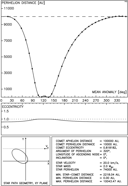 Fig.4.1 Comet perihelion distance after
the stellar passage
Fig.4.1 Comet perihelion distance after
the stellar passage
To present the dependency of the stellar perturbation on the path
geometry it would be necessary to show tens of such plots for different
comet argument of perihelion. Instead of doing this we prepared
different type of plots, where 36 different orientations are presented
in one figure. Such a figure is a composition of 36 different curves
similar to the one presented in the upper part of Fig.4.1. The results
of the same star passage as in fig.4.1 but for different values of
cometary argument of perihelion are presented in Fig.4.2. One can note
that wide regions of large increase and significant decrease of the
perihelion distance are present in this plot.
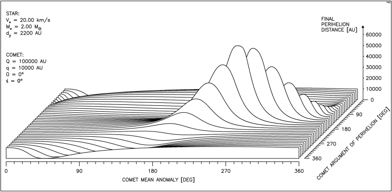 Fig.4.2
Next figures present various cases of the stellar perturbation
applied on comets. All plots show
the final prihelion distance of a comet in dependence of cometary
argument of perihelion and cometary mean anomaly. The parameters of the
star and orbital elements of a comet are presented in the upper-left
corner of each plot. Parameter dy denotes the minimum
star-comet distance. At each particular geometry the minimum Sun-star
distance was adjusted to keep dy approximately constant.
The effect of a typical star passing close to the comet orbit is
presented in Fig.4.3.
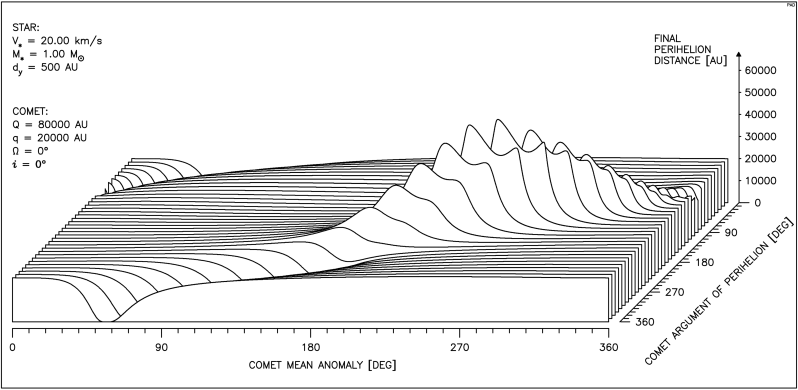 Fig.4.3
The detailed analysis of one of the curves constituting Fig.4.3 is
presented in Fig.4.3a.
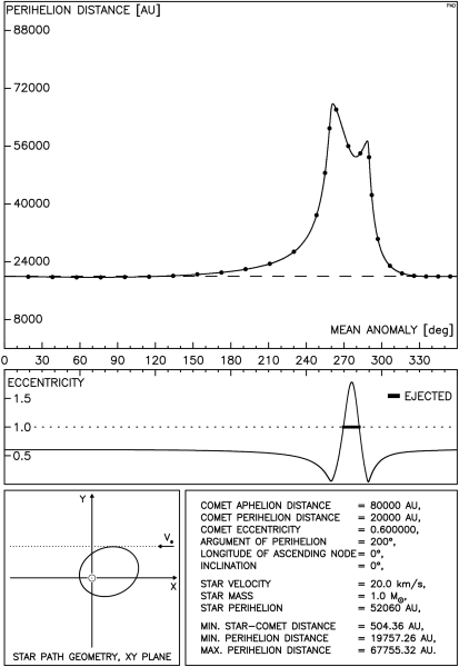 Fig.4.3a.
A case of the strong effect of a massive star is presented in Fig.4.4.
In this case large increase of the perihelion distance are impossible
but the significant decrease are frequent.
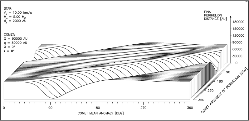 Fig.4.4
A case of the weak perturbation on highly eccentric comet orbit is
presented in Fig.4.5.
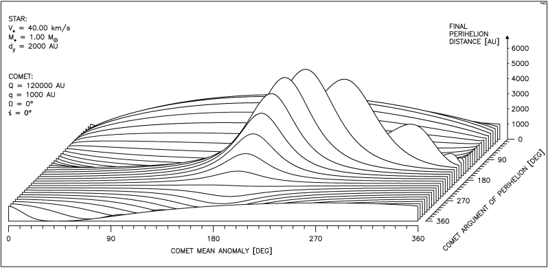 Fig.4.5
The detailed analysis of one of the curves constituting Fig.4.5 is
presented in Fig.4.5a. Please note, that in this case a star moves very
close to the Sun but the improved impulse results are still in
excellent agreement with the numerical integration.
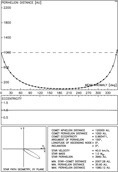 Fig.4.5a.
A case of the low mass and high speed star acting on highly eccentric
comet orbit is presented in Fig.4.6. even such a weak stellar
perturbation can significant change the cometary perihelion distance.
Small values of the argument of perihelion correspond to the wide
region where the solar part of the velocity impulse dominates.
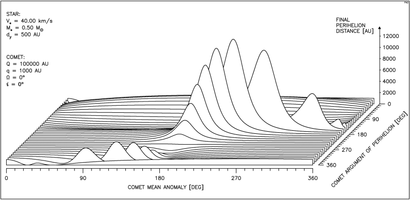 Fig.4.6
The detailed analysis of one of the curves constituting Fig.4.6 is
presented in Fig.4.6a.
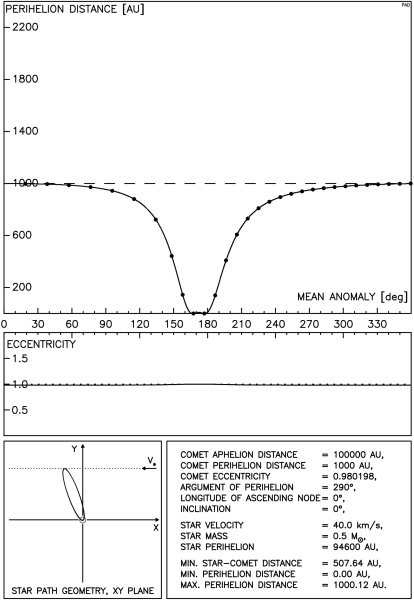 Fig.4.6a.
A case of the high mass and low speed star distant action on highly
eccentric comet orbit is presented in Fig.4.7.
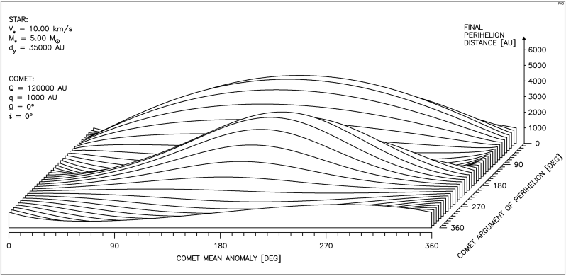 Fig.4.7
The detailed analysis of one of the curves constituting Fig.4.7 is
presented in Fig.4.7a. The observable comet is obtained here despite of
very large comet-star proximity distance.
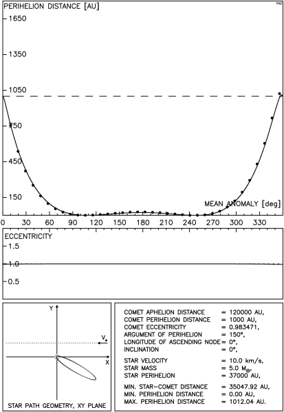 Fig.4.7a.
An extremal case of a very strong stellar perturbation is presented in
Fig.4.8. A massive and slow moving star passes very close to a comet.
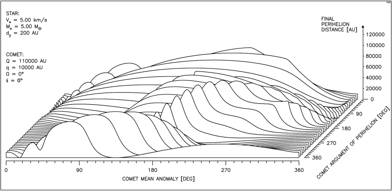 Fig.4.8
The detailed analysis of one of the curves constituting Fig.4.8 is
presented in Fig.4.8a. Small differences between the improved impulse
approximation and the numerical integration are present here.
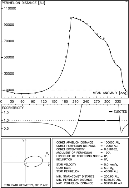 Fig.4.8a.
And another curve from this figure is presented in Fig.4.8b. This is
the only case when the errors of the improved impulse approximation can
be significant. This errors do not result from ignoring the comet
motion as the comet is almost at aphelion. This discrepancies come from
the very small star-comet proximity distance here.
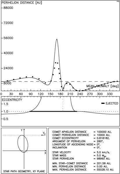 Fig.4.8b.
All result presented so far remain valid also for small inclination
cometary orbits: plots are almost identical.
The plots for cases when a star crosses the comet orbit can be
presented only for a fixed value of the cometary argument of perihelion
(our multiple plots became unreadable).
An example of a star crossing the comet orbit is presented in Fig.4.9.
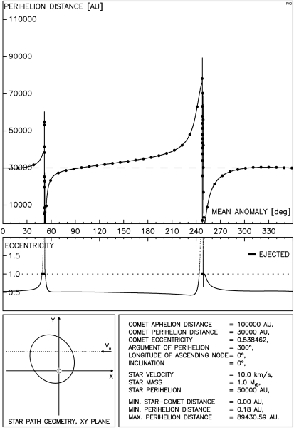 Fig.4.9.
And a closeup of the second crossing is presented in Fig.4.9a. Please
note the excellent agreement of the results from both methods.
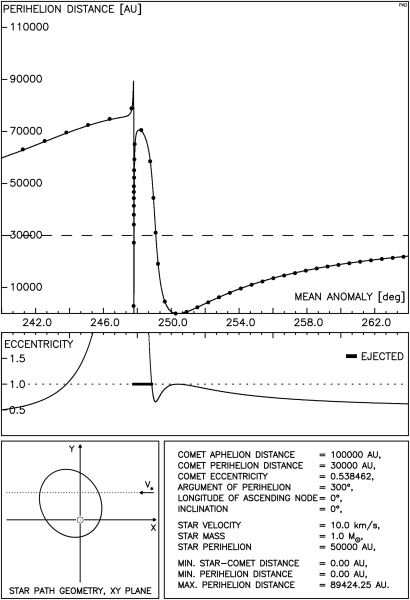 Fig.4.9a.
The example of "grazing" stellar path is presented in Fig.4.10.
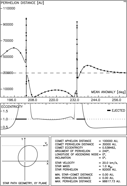 Fig.4.10.
The effect of a massive star crossing an eccentric cometary orbit is
presented in Fig.4.11.
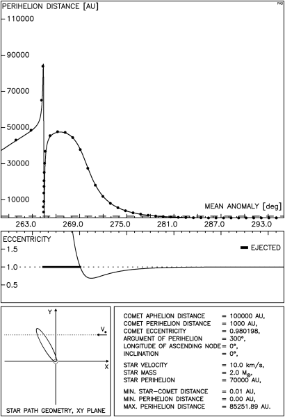 Fig.4.11.
4.2 Comet orbit perpendicular to the stellar path
As in the planar case, the orientation of the cometary orbital plane
remains almost unchanged. The effect of the outer (outside the comet
orbit) and inner (inside the comet orbit) passages gives almost the
same results, as can be seen from Figs 4.12 and 4.12a. A typical star
moves relatively close to the comet orbit.
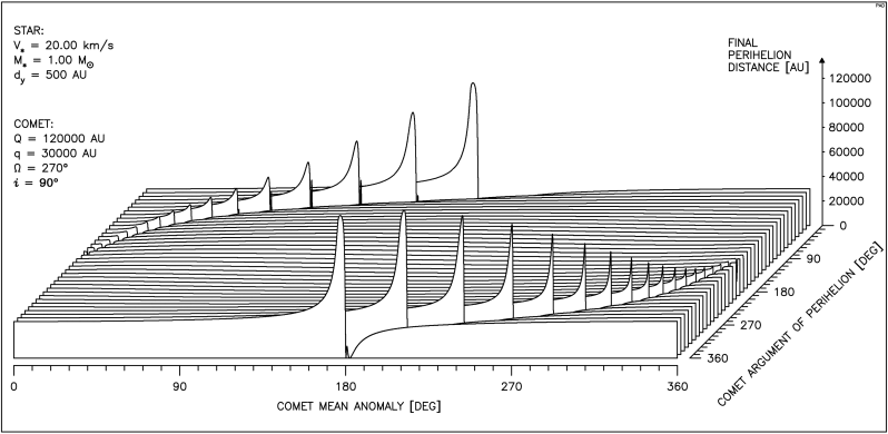 Fig.4.12
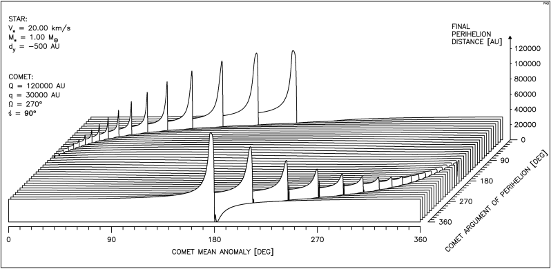 Fig.4.12a
One of the curves from Fig.4.12a is presented in detail in Fig.4.12b.
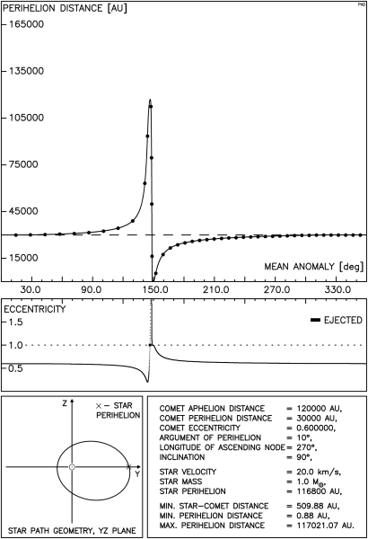 Fig.4.12b
The effect of the massive and slow moving star, acting on low
eccentricity
comet orbit (outer and inner case) is presented in Figs 4.13 and 4.13a.
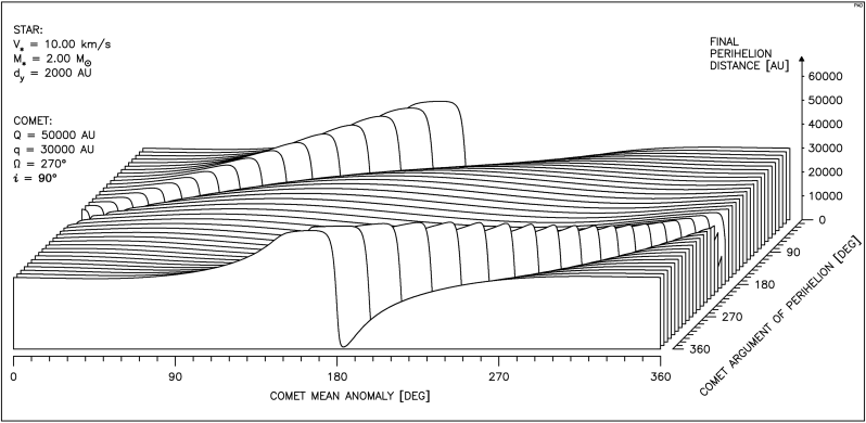 Fig.4.13
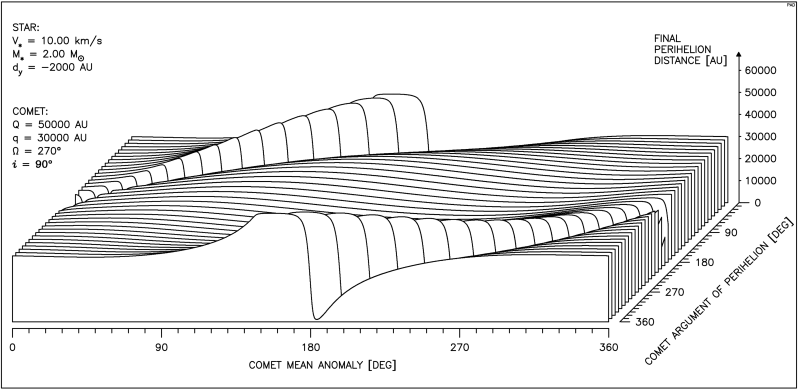 Fig.4.13a
One of the curves from Fig.4.13a is presented in detail in Fig.4.13b.
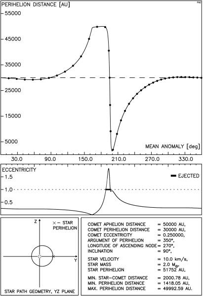 Fig.4.13b
The effect of the massive star, acting on high eccentricity
comet orbit (outer and inner case) is presented in Figs 4.14 and 4.14a.
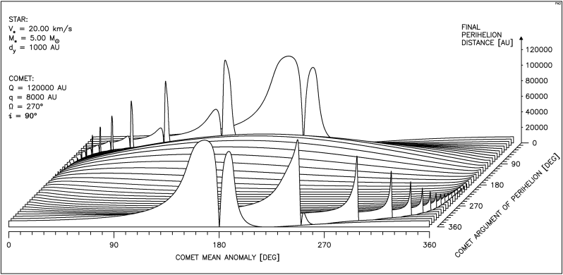 Fig.4.14
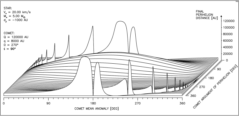 Fig.4.14a
One of the curves from Fig.4.14 is presented in detail in Fig.4.14b.
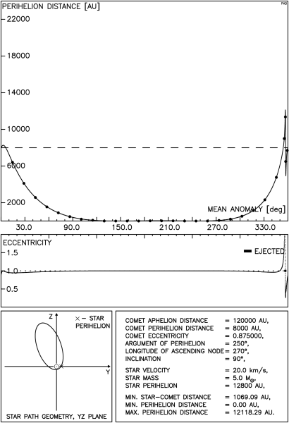 Fig.4.14b
And one of the curves from Fig.4.14a is presented in detail in
Fig.4.14c.
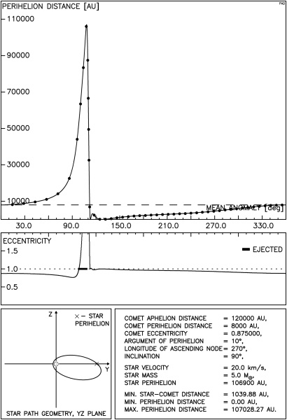 Fig.4.14c
4.3 Other geometrical configurations
Before we present several examples for an arbitrary geometrical
orientation of the stellar path with respect to the comet orbit plane,
we present another example of the perpendicular comet orbit. In all
examples presented in the previous section the minimum comet-star
distance was kept almost constant in particular plot. Now we present an
example of the strong stellar action on the comet with perpendicular
orbit plane but now the star moves closer to the Sun, so the solar part
of the velocity impulse dominates. This can be viewed in Fig.4.15.
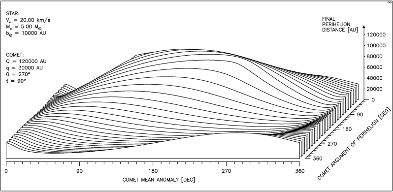 Fig.4.15
One of the curves from this figure is presented in detail in Fig.4.15a.
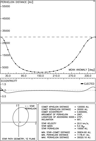 Fig.4.15a
Another curve from Fig.4.15 is presented in detail in Fig.4.15b.
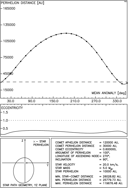 Fig.4.15b
Another example with the solar part dominating but for the stellar path
parallel
to the comet abides line is presented in Fig.4.16.
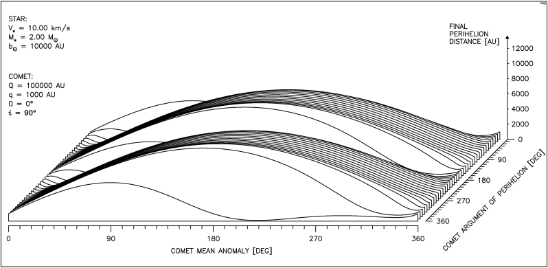 Fig.4.16
One of the curves from this figure is presented in detail in Fig.4.16a.
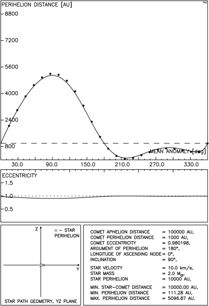 Fig.4.16a
An example of the strong action on the low eccentricity, low
inclination
cometary orbit can be viewed in Fig.4.17.
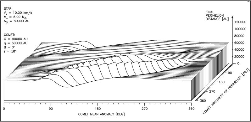 Fig.4.17
One of the curves from this figure is presented in detail in Fig.4.17a.
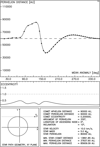 Fig.4.17a
An example of the strong action on the high eccentricity, low
inclination
cometary orbit can be viewed in Fig.4.18.
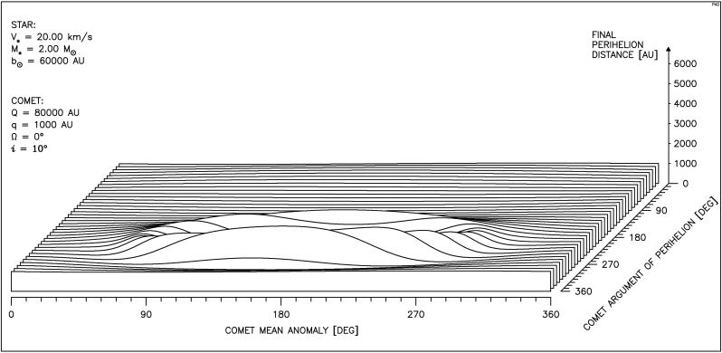 Fig.4.18
One of the curves from this figure is presented in detail in Fig.4.18a.
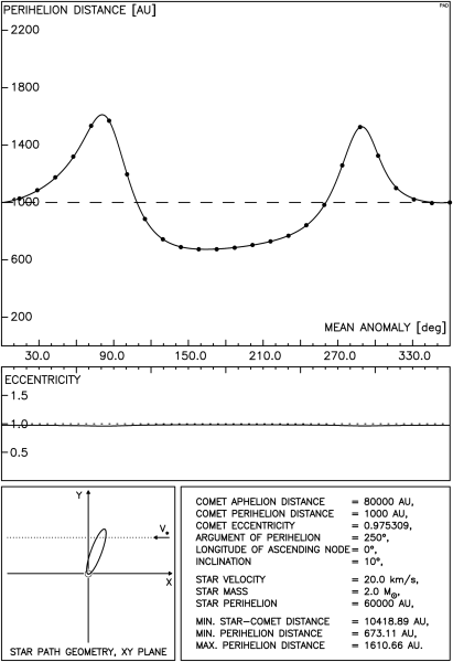 Fig.4.18a
And the last example, a massive and low velocity star moves inside low
eccentricity, high inclination cometary orbit: Fig.4.19.
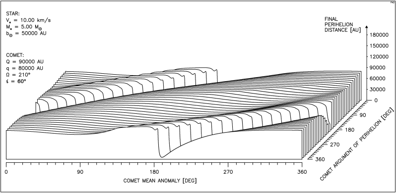 Fig.4.19