Where do long-period comets come from?
26 comets from the non-gravitational Oort spike.
Małgorzata Królikowska1, Piotr A. Dybczyński2
1.Solar System Dynamics and Planetology Group,Space Research Centre, Polish Academy of Sciences, Warsaw, Poland.
2.Astronomical Observatory Institute, A.Mickiewicz University, Poznań, Poland.
ABSTRACT
Since 1950, when Oort published his hypothesis several important new facts were established in the field. In this situation the apparent source region (or regions) of long-period comets as well as the definition of the dynamically new comet are still open questions, as well as the characteristics of the hypothetical Oort Cloud. The aim of this investigation is to look for the apparent source of selected long period comets and to refine the definition of dynamically new comets.
Basing on pure gravitational original orbits all comets studied in this paper were widely called dynamically new. We show, however, that incorporation of the non-gravitational forces into the orbit determination process significantly changes the situation.
We determined precise non-gravitational orbits of all investigated comets and next followed numerically their past and future motion during one orbital period. Applying ingenious Sitarski's (Sitarski,1998) method of creating swarms of virtual comets compatible with observations, we were able to derive the uncertainties of original and future orbital elements, as well as the uncertainties of the previous and next perihelion distances.
We concluded that the past and future evolution of cometary orbits under the Galactic tide perturbations is the only way to find which comets are really dynamically new. In our sample less than 30% of comets are in fact dynamically new. Most of them had small previous perihelion distance. On the other hand, 60% of them will be lost on hyperbolic orbits in the future. This evidence suggests that the apparent source of long-period comets investigation is a demanding question.
We also have shown that a significant percentage of long-period comets can visit the zone of visibility during at least two or three consecutive perihelion passages.
1 INTRODUCTION
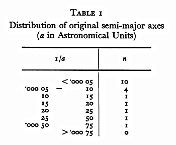
Jan Oort (1950) proposed a hypothesis, that the Solar System is surrounded by a huge, spherical cloud of comets, now called the Oort Cloud. As the argument for the existence of such a cloud he completed a list of 19 original orbits of well observed long-period (hereafter LP) comets and showed, that their inverse of semi-major axis 1/a has the distribution apparently peeked near zero, at the positive side. He concluded that new long-period comets come from distances of 50 000 to 150 000 AU. He also showed, that perturbations by passing stars can change cometary orbit significantly, making it observable as dynamically new long-period comet. During the last 60 years several new factors occurred in this field.
First, the population of precise original cometary orbits increased to several hundreds. In the recently published, 17th edition of the Catalogue of Cometary Orbits (Marsden & Williams, 2008) (hereafter MWC08) 499 precise original and future cometary orbits are listed. Second, new and dominating perturbing force must be included in the model: tidal action of the Galactic disk and Galactic centre. They are negligible when calculating original and future orbits but when following the past or future motion of a comet at larger distances one must take them into account. It means, that looking at the original orbit elements we cannot tell the past or predict the future motion of this body, for example foretell the previous/next perihelion or aphelion distances. This was demonstrated by Dybczyński (2001,2006).
Third, we learned how to investigate and in many cases we can successfully determine non-gravitational forces in the motion of long-period comets. This can significantly change our knowledge of original and future orbits (see for example: Marsden,Sekanina,Yeomans 1973, Królikowska 2001,2006a) It also means, that tens of precise original orbits with determined non-gravitational forces could be added to the MWC08 list.
Taking all this into account, the apparent source region (or regions) of long-period comets as well as the definition of the dynamically new comet are still open questions, as well as the characteristics (if not the existence) of the hypothetical Oort Cloud. In this paper we start to investigate these problems concentrating on 26 comets constituting so-called non-gravitational (hereafter NG) Oort spike, i.e. having 1/aori,NG < 10-4AU-1. This particular choice comes from the fact, that after applying non-gravitational model in orbit determination we obtain significantly different distribution of the inverse original semi-major axes. Almost all 1/aori values were shifted to larger values and among them a lot of hyperbolic cases changed into elliptic ones. Since we want to study the implications of obtaining non-gravitational original orbits on the Oort hypothesis, the past (and future) motion of these 26 comets were analyzed at first.
In Section 2 we describe observational material and its processing. In the next section calculation of original and future cometary orbits for the selected 26 non-gravitational Oort spike comets is described in detail. Section 4 describes the numerical integration of the past and future motion of these comets under the action of Galactic tides. Then, results and conclusions are presented.

| 
|
| Fig.1 The O-C distributions for Comet C/C/2004 B1 LINEAR and C/2001 Q4 NEAT. The non-weighted data are presented in the left-side column for each comet and the weighted data – in the right column where the gravitational cases are displayed in upper figures and the NG cases in lower figures. The best-fitting Gaussian distributions are shown by magenta dots, each chosen exactly in the middle of histogram bin. | |
2 OBSERVATIONS AND THEIR PROCESSING
MWC08 includes 184 comets with 1/aori < 10-4AU-1 where for majority of them the orbits are determined with the highest accuracy. At first we looked at 154 most precise orbits. Thus, we took into account all comets with the quality class 1 according to the classification introduced by Marsden et al. (1978). About half of them have perihelion distances less than 3.0 AU, what means that we should suspect detectable influence of the non-gravitational forces. The inverse dependence of the strength of non-gravitational forces on the perihelion distance is widely expected and indeed is clearly visible in our Fig.5 (to be described in detail in the next section). We took into account almost all these objects (except ten comets discovered before 1950 where positional data were not available for us) and additionally all LP comets with the NG orbits in MWC08 (29 objects, 1/aori are not given for them in the Catalogue). In majority of cases, the observational material taken for orbital determinations is more complete than in the MWC08: for comets from the XIX century the observations were collected directly from the published papers, for comets from the first half of XX century the data were collected in Warsaw in cooperation with the Slovakian group at the Astronomical Institute in Bratislava and Tatranska Lomnica, more modern data were taken from the Minor Planet Electronic Circulars available through the Web Page at http://www.cfa.harvard.edu.
Table 1.Observational material
for 26 comets under consideration
(click the table for the enlarged version).
From these class 1 objects we were able to derive the sample of 26 LP comets with determinable non-gravitational effects from the astrometric data and with the non-gravitational reciprocals of semi-major axes not greater than 10-4AU-1 (1/aori,NG <10-4AU-1, hereafter: NG Oort spike). Among them only 9 comets(C/1885 X1, C/1956 R1, C/1959 Y1, C/1986 P1-A, C/1989 Q1, C/1990 K1, C/1993 A1, C/2001 Q4, C/2002 T7) have NG orbits presented in MWC08. C/1990 K1 Levy has formally 1/aori,NG slightly greater than the adopted limit but the uncertainty interval of it evidently overlap with the NG Oort spike defined above. We have not included in our sample objects which are still potentially observable because the derived orbits for these objects could not be treated as definitive results. The preliminary investigation of the original non-gravitational reciprocals of semi-major axes 1/aori,NG are given in Królikowska (2006) for the majority of these 26 comets. In that paper data have not been weighted, while now, to obtain the more reliable orbits, we decided to include the weighting of observations into the data processing.
The determination of the NG parameters in the motion of LP comets is very difficult mainly due to limited observational material covering one apparition or even just half apparition (in the case when comet was discovered after its perihelion passage). Thus, the processing of astrometric data is crucial for this purpose. Królikowska (2006) divided each set of astrometric data into preperihelion and post-perihelion arc (when it was possible) and then selected data in each part independently. The difference of rms for the whole data set (for the pure gravitational solution) and the rms obtained separately for both parts of the orbit indicates how strongly the NG-effects affect the orbital motion. After many tests we have recognized, however, that the weighting is crucial for the orbit fitting for comets discovered before 1950 and sometimes for modern comets, too. Thus, we decided to adopt more advanced data treatment. Each set of astrometric data has been processed individually for the pure gravitational orbit and non-gravitational case independently in the following way.
For each comet we tested two methods of selecting and weighting data for both: pure gravitational and non-gravitational orbit, independently. It means that we determined four nominal solutions for each object: two for pure gravitational case and two for non-gravitational case (based on different data treatment). It allows us to choose the best and as homogeneous as possible data processing for the whole sample of LP comets. We tried to use the most but reasonable discriminative selection criterion and according to our tests the year 1950 can serve as a suitable dividing date. Thus, we divided all considered comets into two sets: comets discovered before and after 1950. These two sets of observations were refined independently for gravitational and non-gravitational orbit determination by applying
- for comets before 1950:
- Chauvenet's criterion for selection procedure + weighting,
- Bessel's criterion for selection procedure + weighting,
- for comets after 1950:
- independent Bessel's selection for observations before and after perihelion, no weighting,
- Bessel's criterion for selection procedure + weighting.
To reduce systematic errors in the observational material, such as the bias associated with a site as a function of time, one should consider specific procedures. For example, in the case of long sequences of observations we divided the whole observational material into a few time subintervals according to the internal structure of material, i.e. according to the existing gaps in observations.

Fig.2 The O-C diagrams for Comet C/1997 J2 Meunier-Dupouy
(weighted data). Two upper figures are given for O-C based on pure gravita-
tional solution, two lower - for O-C based on NG solution. Residuals in right
ascension are shown as magenta dots and in declination as blue circles;
the moment of perihelion passage is shown by dashed vertical line.
The data of two comets with the number of observations less than 100 (C/1952 W1 and C/1959 Y1) have not been weighted. For two of the comets discovered before 1950 the Chauvenet's and Bessel's criterions gave the same set of residuals and for the next three comets the differences in the number of rejected residuals are very small (less than 1%). Thus, we present here results derived for more discriminative Bessel's criterion also for comets before 1950. One should note that our data processing resulted in reasonably low number of rejections (below 17% - for comets before 1960 and with mean percentage of rejected data of 3.4% - for comets after 1960; the only extreme case here is C/C/2004 B1, for which 9% of observations was rejected). The description of observational data used for orbital determination is presented in Table 1 where comets are ordered by discovery date.
To determine the NG cometary orbit we used the standard formalism proposed by Marsden et al. (1973) where the three orbital components of the NG acceleration acting on a comet are symmetric relative to perihelion:

where F1, F2, F3 represent the radial, transverse and normal components of the NG acceleration, respectively. The exponential coefficients m, n, k are equal to 2.15, 5.093, and 4.6142, respectively; the normalization constant α = 0.1113 gives g(1 AU) = 1, the scale distance ro =2.808 AU. From orbital calculations, the NG parameters A1, A2 and A3 were derived together with six orbital elements within a given time interval (numerical details are given in Królikowska 2006). This NG model assumes that water sublimates from the whole surface of an isothermal cometary nucleus. One can see in the 10th column of Table 2 that in some cases just two NG parameters were determinable with reasonable accuracy (in two cases – only one NG parameter). We decided to use in this investigation the minimal necessary number of NG parameters. For example, in the case of C/1993 A1 and C/1996 E1 the NG parameter A3 is determinable, however, the decrease of rms (relative to NG solution with A1 and A2) is insignificant with no perceptible changes in OC diagrams and O-C distributions (compare with online material in Królikowska (2004)). The asymmetric NG model which introduces the additional NG parameter τ - the time displacement of the maximum of the g(r(t-τ)) relative to perihelion, seems be important just for one comet, C/1959 Y1 Burnham, what makes the number of NG parameters for this comet to be equal 4.

Fig.3 The O-C diagrams for Comet C/2001 Q4 NEAT (weighted data).
Two upper figures are given for O-C based on pure gravitational
solution, two lower – for O-C based on NG solution (for the clarity
the three last observations taken in August 2006 are not displayed).
Symbols have the same meaning as in Fig. 2
To decide whether the derived NG solution better represents the actual motion of individual comet than the pure gravitational orbit we use three criterions:
- decrease of the rms for the NG solution in comparison with the pure gravitational solution,
- smaller trends in O-C diagrams for NG orbit fitting,
- the O-C distribution of NG orbit closer to the normal one.
After inspection of the O-C diagrams and distributions we always conclude that the NG orbit derived from the weighted and selected data sets represents the actual comet motion much better than the pure gravitational orbit. This fact is visualized in Fig.1 for two comets C/C/2004 B1 and C/2001 Q4. Therefore, the pure gravitational orbits are presented in this paper only for comparison and to show that such orbits could produce misleading orbital results and incorrect conclusions about future and past history of cometary dynamics. The examples of differences in the O-C diagrams between pure gravitational and NG solutions are presented for two comets in Fig.2 and Fig.3. For comet C/1997 J2 only pure gravitational orbit is presented in MWC08 as well as at the JPL Small- Body Database Browser (http://ssd.jpl.nasa.gov/sbdb.cgi), whereas for Comet C/2001 Q4 NG solutions are presented in both sources. Fig.2 reveals that some trends visible in pure gravitational O-C diagram for C/1997 J2 Meunier-Dupouy are almost canceled for NG solution while the rms decreased from 0.0091 to 0.0067. Similar behavior was noticed for all NG solutions given in this paper even for four objects with largest perihelion distance (q>3.0 AU) as was shown in Fig.2 for Comet C/1997 J2.
Among investigated sample of NG Oort spike comets C/2001 Q4 NEAT presents the case of one of the most significant decrease of rms from 1.29 (pure gravitational orbit, non-weighted data) to 0.63 (NG orbit, weighted data) (Table 2, Fig.1, Fig.3 ). In this group are also C/1959 Y1 Burnham, C/1990 K1 Levy, C/1993 A1 Mueller and C/2002 T7 LINEAR.

| 
|

| 
|
| Fig.4 Projection of the 6D/8D space of 5 000 VCs of C/1989 Q1 (upper panel) and C/1993 A1 (lower panel) onto the e-q plane. Left plots show the pure gravitational swarms of VCs, right plots – NG swarms. Each point represents a single virtual orbit, while its colour indicates the deviation magnitude from the nominal orbit with the confidencelevel of: < 50%, 50% - 90%, 90% - 99%, and > 99% (from red, through magenta, blue to cyan points, respectively). Each plot is centered on the nominal values of respective pair of osculating orbital elements denoted by the subscript 'o'. | |
For many comets with evidently detectable NG-effects we obtained strongly non-Gaussian O-C distribution for pure gravitational orbit whereas the O-C distribution follows the normal distribution when the NG orbit were fitted. An excellent example of such behavior is Comet C/C/2004 B1. The departures from the best Gaussian fitting to O-C residuals are shown in Fig.1. One can note that the deviations of O-C distribution from normal distribution in the pure gravitational case always decreased for weighted data in comparison to non-weighted data, however in some cases this deviation is still clearly visible even for weighted data as one can see for both comets presented in Fig.1. It seems evident that non-Gaussian distribution of O-C residuals results from ignoring of NG forces in the cometary motion. In a few cases (C/1990 K1, C/1993 A1, C/2001 Q4, C/2002 T7 and C/C/2003 K4), however, the O-C distributions for NG solution obtained on the basis on weighted data differ from the Gaussian distribution also. In all these five cases the residuals in NG model still display some trends too (especially around perihelion passage), though less significant than in the pure gravitational case (Fig.3). We tested that the time-shifted g(r)-function relative to perihelion passage do not improved the O-C diagrams here. It seems that some other function than standard g(r) would be more adequate to describe the NG effects in these comets. It should be noticed, however, that the presented NG nominal orbits for these five comets are closer to actual cometary orbit than pure gravitational solutions.
And the last, important remark concerning the gravitational solutions determined from weighted data. In practice, these solutions are not purely gravitational since the time distribution of weights could compensate the NG trends. For three objects from our sample (C/2002 T7, C/2001 Q4 and C/1997 BA6 ) relative decreasing of rms and some time-dependence in weights are evidently visible . For the most spectacular case (C/2002 T7) the rms of gravitational solutions decreased from 1.21 arcsec (non-weighted data) to 0.61 arcsec (weighted data) whereas the rms of NG solutions decreased from 0.64 arcsec to 0.58 arcsec, respectively, and systematic trends in weights disappeared. Thus, we should keep in mind that so called gravitational solutions determined on the basis of weighted data could partially incorporate NG trends.
3 OBTAINING THE MOST PROBABLE ORIGINAL AND FUTURE ORBITS
Table 2.Original and future semi-major axes derived from pure gravitational nominal solutions (columns 2–3) and NG
nominal solutions (columns 4-5) where the number of NG parameters determined for NG solutions is given in the
column 10. The rms's and number of residuals are given in the columns 6-7 and 8-9, respectively, where 'GR' refers
to gravitational nominal solution. If there are two rows for a particular comet, the first describes results with
weighting and the second without weighting. Single row (older comets) means that weighting was applied.
There is an extended version of Table 2 available on-line
To investigate the past and future history of each particular comet we have examined the evolution of thousands of virtual comets (VCs) orbits from the confidence region, i.e. the 6-dimensional region (7-9D region in the NG case) of orbital elements (and NG parameters), each time fully compatible with the observations. We constructed the confidence region using the Sitarski's method of the random orbit selection (Sitarski 1998).
This method allows us to generate any number of randomly selected orbits of VC. It should be noticed that according to this random selection method the derived sample of VCs follows the normal distribution in the orbital elements space (also the rms's fulfil the 6-9 dimensional normal statistics; Królikowska et al. 2009).
In the calculations described here we fill a confidence region with 5 000 VCs for each nominal solution (GR and NG) for each considered comet. Fig. 4 shows projections of the 6D/8D parameter space of 5 000 VCs of C/1989 X1 (upper panels) and C/1993 A1 (lower panels) onto the plane of two chosen orbital elements. Orbital cloning procedure was applied close to the observational arc (at the epoch of 1990 April 19 and 1992 October 25, respectively). The derived swarm of VCs follows the normal distribution in the 6D space of orbital elements (8D space of orbital elements and two NG parameters in the NG case for both comets). This is visualized by four grey tints of points inFig. 4. Each point represents a single VC, while its grey tint indicates the deviation magnitude from the nominal orbit with the confidence levels defined as follows: < 50%, 50% - 90 %, 90% - 99%, and > 99% (from the darkest to brightest points, respectively). The symbols in crowded areas heavily overlap and the brighter points are often overprinted with darker ones. One can see that the NG swarm of C/1989 X1 is more disperse than its pure gravitational swarm (upper panel of Fig. 4). Similar situation took place in almost all investigated comets except C/1993 A1 and C/2000 SV74 . The largest dispersion of original NG swarm within our sample of NG Oort spike comets appeared in case of comet C/1959 Y1 Burnham where four NG parameters were determined. In the C/1993 A1 case the compactness of NG swarm of VCs is higher than compactness of GR swarm though in the first case we determined two more parameters from the same data set than in the latter case (lower panel of Fig. 4). It is a consequence of radically better NG orbit fitting to data (rms=0.98 arcsec) in comparison to pure gravitational orbit fitting (rms=2.49 arcsec). In the majority of cases, however, the relative decreasing of rms is smaller and the NG swarm of VCs is more disperse than pure gravitational swarm, as expected when increasing parameter space dimensions.

Fig.5 Shifts of 1/aori due to the NG effects for 26
of investigated comets. Three largest uncertainties of
1/aori;NG belong to comets C/1959 Y1 and C/1952 W1
and C/1892 Q1 (see also Table 2 and section 5.3.3).
To calculate the original and future swarm of cometary orbit each of VC was followed from its position at osculation epoch backwards and forwards until the VC reached a distance of 250 AU from the Sun. The equations of comet's motion have been integrated numerically using the recurrent power series method (Sitarski 1989, 2002), taking into account perturbations by all the planets and including the relativistic effects. In this way we were able to obtain the nominal original/future orbit of each comet as well as the uncertainties of the derived values of orbital elements by fitting the normal distribution to each original/future cometary swarm (Królikowska 2001). Original and future semi-major axes with their uncertainties are given in Table 2 where comets are ordered by discovery date. Fig. 5 visualizes the differences between original 1/a derived for NG and GR swarms of comets. One can note that all investigated comets have 1/aori,GR < 5×10⁻⁵ AU-1. This means, that all these comets would belong to the first row of Table 1 in the Oort (1950) paper.
4 PAST AND FUTURE MOTION UNDER THE GALACTIC TIDE
4.1 Force model
Following Fouchard et al. (2005) and others, we used a set of equations of motion in the vicinity of the Sun, accounting for Galactic disk tide and Galactic centre tide. Prętka (1998, 1999) argued that for relatively small time intervals (say ten million years) it is not necessary to include the Galactic centre term, as its influence manifests significantly on considerably longer time intervals. However, to maintain compatibility with other works in the field and taking into account, that including Galactic centre term into the model of Galactic tides is not very time consuming we decided to use such a full model. During all integrations we performed calculations in both: simplified and full Galactic tide models, just to confirm the above-mentioned conclusions and observe the difference in some specific cases. It appeared, that while qualitative evolution is almost the same, the quantitative results may differ. Some examples of the significant differences in the output from these two models are given in Figs.6 and 7.
We use here two different frames. The rotating frame is defined as a heliocentric frame with the X' axis in the radial direction pointing toward the Galactic center, the Y' axis pointing along the Suns velocity, and Z completing a right-handed system. The nonrotating frame OXYZ coincides with this rotating one at t = 0, but keeps its direction fixed. Basing on Heisler & Tremaine (1986) one can write the formula for the tidal force from the disk and the centre of the Galaxy in the rotating galactic frame OX'Y'Z' as follows

where A and B are the Oort galactic constants, G is the gravity constant, r is the heliocentric distance, ρo is the local disk matter density and MB is the central mass (the Sun and planets), expressed in solar masses. Let G1, G2 and G3 be such that:

then the equations of motion in rectangular coordinates (OXYZ inertial frame) are:

where Ωo is the angular velocity of the Sun about the Galactic center and as a consequence the angular velocity of the rotating frame with respect to the nonrotating one and

Substituting this into the equations of motion and remembering that G2 = -G1 (all contemporary models of Galactic tides adopt B2 = A2 , see Fouchard et al. (2005) as the most recent review of the different tide models and their calculation methods) we obtain:


Fig.6 The comparison of the past motion of C/C/2003 K4 for
different force-models. The blue line depicts the swarm
of VCs stopped at previous perihelion when full Galactic
tide (disc + centre) was used. The red line is for simplified
(disc only) model. For the comparison the starting swarm
(very concentrated in this scale) is shown in the right,
lower corner with black dots. For each swarm the
nominal comet orbit is situated at the centre of the
corresponding green circle.
which is the set we integrate numerically. We used G1 = -7.0702403×10⁻¹⁰, and G3 = 4πGρo, where ρo , is the local Galactic mater density in solar masses per cubic parsec. The model limited to the disk tide can be obtained by putting G1 = 0, and we used it in parallel, to monitor the separate influence of the Galactic centre term. Two examples of such a comparison of different dynamical models are presented in Figs. 6 and 7. As it concerns the adopted value of the local Galactic mater density ρo , we followed most of the contemporary papers in the field, adopting ρo = 0.100 solar masses per cubic parsec.To observe the influence of a possible error in this value we repeated the calculations for several comets using three significantly different values: ρo = 0.050, ρo = 0.100 and ρo = 0.150 solar masses per cubic parsec. An example of such a comparison is presented in Fig.8, which is significantly magnified to make the differences visible.

Fig.7 The comparison of the past motion
of C/1986 P1-A for different force-models.
All symbols have the same meaning as in Fig.6.
Dybczyński (2006) have shown, that none of the known stars could significantly influence the cometary motion recently (during last 10 million years, or so) and in similar time interval in the future. This time interval is comparable with orbital period of an elliptic comet with the semi-major axis of 50 000 AU and thus it is close to the timescale of the longest past or future cometary motions analyzed in this paper. Dybczyński (2006) searched for real stellar perturbers in all available catalogues, selected several stars with maximum possible influence on the Oort cloud comets and showed that comparing with Galactic perturbations their influence is negligible. He also presented a discussion on the completeness of the stellar data (besides positions, both parallax and radial velocity are necessary). In short: we cannot be sure that some stars passed (or will pass) in the vicinity of the Sun during 20 million years time interval, centred at present. But these stars are absent in our catalogues either because they are too small (e.g. brown dwarf, see for example: Research Consortium on Nearby Stars 2009) or move very fast, and now are too far, or both. But only relatively massive stars (of order of one solar mass or more) and moving rather slowly (less than 30 km s-1) can significantly change cometary orbit, even with the aphelion at 100 000 AU. For more detailed discussion see Dybczyński (2006).
For the reasons explained above, and taking into account, that precise calculation of (even very weak) stellar perturbations would be time consuming, we decided to omit them in our model. Perhaps in future, especially if some important star will be discovered (and its parallax and radial velocity will be measured, see Dybczyński & Kwiatkowski 2003) we will include its gravitational influence on the Sun and a comet into our model.

Fig.8 The comparison of the future motion of C/1996 E1 with
three different ro values used. The full Galactic tide model was
used here and all VCs were stopped at 120 000 AU, going out
of the Solar System. The blue swarm was obtained for
ρ = 0.050 solar masses per cubic parsec, the red one
was obtained for nominal value ( ρ =0.100 solar masses
per cubic parsec) and the black one for ρ =0.150 solar
masses per cubic parsec. The centre of the green circle
drawn on top of each of the swarms denotes the position
of the nominal comet orbit.
4.2 Numerical integration
The original and future orbit calculations produced an output in the form of a set of 5001 (nominal orbit plus 5000 VCs) barycentric orbits for each comet under consideration. To observe how Galactic perturbation action varies depending on small initial condition changes we separately followed numerically all 5001 VCs, in general, one orbital period to the past and to the future. We used the well known, widely used and tested routine RA15 (Everhart 1985) with the force model described above (with the parameter LL=12 to obtain the highest possible accuracy on 64-bit computers). Since the Galactic tide is relatively weak, the automatically adjusted integration step was generally very large so the speed of the calculation allowed us to follow individually such a big number of VCs for each comet.
Since we are interested mainly in the past motion of a comet and the apparent source of the observed long-period comets we followed their past motion for one orbital period. Having the opportunity to investigate also the future motion of these bodies we decided to perform similar calculations for all of them going one orbital period to the future. Going further (both back and forth) seems useless, since a lot of comets have their previous and/or next perihelion distances deep in the Planetary System. Since there are no means to calculate precise planetary perturbations for such bodies say ten million years from now, we cannot follow their motion "behind" previous and/or next perihelion point. On the other hand, when a comet have large previous/next perihelion distance, their subsequent motion do not change our knowledge on the apparent source of the observed long-period comets, or their future.
The situation complicates when past or future orbit of particular VC is hyperbolic. We have to stop numerical integration at some heliocentric distance, which we call escape limit. To define this limit it seems useful to recall contemporary studies on the outer border of the Oort cloud. Among recent reviews in this field we mention a chapter in Comets II book by Dones et al. (2004) and a book by Fernández (2005). Both present consistent conclusions that while Oort placed the outer border of the cometary cloud at 5-15×104 AU current understanding of cometary dynamics makes this border much smaller, say 2-8×10⁴ AU for the aphelion distance and 1-4×10⁴ AU for semi-major axis. Additionally, the majority of the observed Oort spike comets have the semi-major axes in the range of 20 000 - 50 000 AU for pure gravitational orbits but this significantly decreases to the value less than 20 000AU if the NG forces are included in the dynamical model. Some discussion of this effect is also in Section 5.2.

Fig.9 The past motion of C/2002 T7. Presented here is
the distribution in q-e plane of all 5001 VCs for that
comet, stopped at previous perihelion. One can see that
the distribution of the previous perihelion distance is very
close to the Gaussian one. In the center of the green circle
the nominal orbit is located.
We decided to be very careful (and a little conservative) so we decided to adopt the escape limit to be equal 120 000AU. This is the maximum heliocentric distance (or maximum aphelion distance) at which we still follow every VCs motion. This was also applied for very elongated elliptic orbits; if the particular VC goes further than 120 000AU from the Sun we call it escaping and stopped the numerical integration.
This particular choice of the escaping border was unfortunate for a handful of comets, where small number of VCs traveled a little bit further than 120 000 AU, but then return to the Sun. We examined closely all such cases and if the necessary increase in the outer limit seemed acceptable we changed it to obtain homogeneous swarm of returning VCs for that particular comet. Such a procedure was applied for example for C/1996 E1, where increasing the outer limit up to 140 000AU allowed all 5001 VCs to return to their previous perihelion among Solar System planets when calculating its past motion. To obtain the same effect for C/1885 X1 one should extend the outer limit up to 260 000AU, what, in the light of arguments included in both papers quoted above, seems problematic. At such a large heliocentric distance the comet motion became chaotic, see Fig. 1 in Dybczyński (2001).
Due to the fact, that some VCs swarms consists of both returning and escaping ones, the rules of stopping the integration were sometimes more complicated: the escaping part of the swarm was stopped at the 120 000 AU and the rest of VCs was allowed to reach previous/next perihelion. There were also a synchronous variant of calculation stopping: for returning swarms all VCs were stopped when the nominal one reached previous/next perihelion and for escaping or "mixed" swarms, all VCs were stopped when the fastest escaping VC reached 120 000AU. This was done to obtain more homogeneous swarm to analyze, where all VCs are stopped at the same time.

Fig.10 The past motion of C/1989 X1. Presented here is the
distribution in q-e plane of 4974 returning VCs for that comet
(black dots), stopped at previous perihelion and 27 escaping
(while still elliptic) VCs - dark grey (red) dots. One can see
that the distribution of the previous perihelion distance is
significantly different from the Gaussian one. In the center
of the dashed-line circle the nominal (returning in this case)
orbit is located. See text for additional explanation.
5 RESULTS
5.1 Overview
Let us start with the context, in which our results should be interpreted. In his paper, Oort (1950) treated original semi-major axes as definitive for describing past motion of a comet. In the same time he stated, that all comets with 1/aori < 1×10⁻⁴ AU-1 should be treated as dynamically new, i.e. they are visiting the observable region for the first time. Such a conclusion came from two assumptions. First, the only possible perturbation source are stellar perturbations, what means that going to the past we should follow original, unperturbed orbit as long as a comet reaches the heliocentric distance large enough to be perturbed by passing stars. Second, all observed long-period comets were significantly perturbed by stars (if not, their keplerian, original orbits bring them exactly to the same perihelion distance at previous passage and no one can call them "dynamically new").
Today, none of this two assumptions seem to be fully correct. As we noted in the Introduction, a comet motion now cannot be treated as unperturbed and the dominating (if not the only one) perturbing force is the differential, gravitational action of our Galaxy. While Galactic tides perturb the semi-major axis practically on the negligible level during one orbital period, the most important part of the past and future cometary orbit evolution manifests in the eccentricity changes.
As a result, while semi-major axis remains almost unchanged, the perihelion distance can change significantly, even during one orbital period both in past and future motion of course. Taking C/1913 Y1 as typical example, one can note that the original semi-major axis of this comet a=19022.723AU and one orbital period before it was equal 19022.794AU. At the same time original perihelion distance q=1.10AU and one orbital period earlier it was equal 2.30AU. Small changes in the semi-major axis under the Galactic perturbations is a well known fact. In the averaged problem of the disk tide the semi-major axis is even an integral of motion (see Breiter et al. (1996) for details). Prętka (1998, 1999) showed that slow secular changes in the semi-major axis due to the action of the Galactic centre can be observed on the much longer time intervals than considered here. It means that looking only at 1/aori of a comet nobody can say what was its previous (or next) perihelion distance.
5.2 Past and future evolution - some statistics
Table 3. The past distributions of the NG swarms of VCs in terms of returning [R], escaping [E], including hyperbolic [H]
VC numbers; the rule of discriminating between [R] and [E] are explained in section 4.2. Aphelion and perihelion
distances are described either by a mean value for the normal distributions, or three deciles at 10%, 50% (i.e. median),
and 90%. In case of mixed swarms the mean values or deciles of Q and q are given for returning part of the VCs swarm.
For comparison we included the osculating perihelion distance in the second column. Last two columns present the value of
1/aori and the percentage of VCs, that one can call dynamically new, basing on previous q statistics.
a – this part of swarm includes the nominal orbit, b – 12 VCs have 200 000AU <Q<320 000AU and 3 VCs - Q between
0.4 - 6.1×10⁶ km, c – we used 140 000AU as the outer border (just 6 VCs have Q>120 000AU).
There is an extended version of Table 3 available on-line
As it was described in sections 2, 3 and 4, we very carefully determined orbits for 26 observed long-period comets using sophisticated observations treatment and NG force model. Than, at osculating epoch, we created 5000 VCs for each comet and precisely propagate all 5001 massless bodies back and forth in time to the limit of planetary perturbations. Todorovic-Juchniewicz (1981) showed that the planetary perturbations in the comet’s motion should be included up to 150 - 200 AU. Thus, we chose 250 AU as safely distant limit where Galactic perturbations are still negligible. Next, we followed numerically past and future motion of each comet swarm (consisting of nominal orbit and 5000 VCs) under the influence of Galactic tides. We stopped the calculation either at past/future perihelion or when the body in question crosses the assumed "escape" border, defined at 120 000 AU.
The results of the investigation of past motion of all 26 comets are summarized in Table 3, while the same for future motion is shown in Table 4. We present here only results for NG model as we are convinced that they gives better description of real cometary orbit and its evolution. For sake of comparison we prepared extended version of Tables 3 and 4 consisting of GR and NG results and their propagation end-states, but due to the volume of information, this is available as the on-line material accompanying this paper only (Dybczyński & Królikowska 2009). Table 3 presents the most important result of this paper. For each comet we show, how many VCs return to previous perihelion (column [R]), how many cross the adopted escape border at 120 000 AU ([E] column) and additionally how many of escaping VCs have formally hyperbolic orbits at the end of our calculation ([H] column, which presents subset of [E] column). Next three columns are discussed below. Last column shows the percentage of VCs, that one can call dynamically new, basing on previous perihelion distance statistics, i.e. we calculate the part of dynamically new VCs by adding the number of returning VCs with qprev >15AU to the number of escaping VCs. It is remarkable that none of the comets from our sample can be called for sure hyperbolic before they enter the sphere of visibility. Three of them, namely C/1982 Q1, C/1952 W1 and 1959 Y1 have significant (but always less than 50 % of all VCs) percentage of hyperbolic VCs and only one, C/1952 W1 have formally negative solution for the inverse semimajor axis: 1/a = (-0.1±85.8)×10-6 AU. However, this value was determined with the largest relative uncertainty, what results mainly from the smallest number of observations.
For 15 comets all 5001 VCs are returning and for additional 5 there is only small (or very small) percentage of escaping VCs, constituting typical long tails of a broad distribution.

Fig.11 The same swarm of VCs for the comet C/1989 X1,
but all were stopped synchronously when the fastest escaping
VC reached 120000 AU. Number of returning and escaping
VCs is the same of course (4974 and 27, respectively).
See text for additional explanation.
For each of 26 comets investigated here we obtain all or significant percentage of returning VCs in their past motion. Thus, we were able to present previous aphelion and perihelion distances statistics for the returning part of each swarm, see Table 3. In small number of cases when the distribution remains Gaussian we present its mean value and standard deviation. An illustration of such a case is given in Fig. 9. However, in the majority of cases the nonlinear action of the Galactic tide have deformed the distributions and they cannot be approximated with the Gaussian distribution. In such cases we decided to describe these distributions by three deciles, namely values separating 10%, 50% (median value) and 90% of all VCs for a particular comet. An example of the non-Gaussian distribution is given in Fig. 10. Here 4974 VCs are returning (black dots). The strange placement of 27 escaping VCs (dark grey or red dots) is caused by the fact, that they were stopped at 120 000 AU border, while returning VCs were stopped at previous perihelion, much later. If we stopped all 5001 VCs synchronously, when the fastest escaping VC reached 120 000 AU the distribution of VCs in the q - e plane will be quite different, what can be seen in Fig. 11.
The most complicated cases occur when the swarms of VCs divides into two distinct parts: returning and escaping (very often with significant number of hyperbolic past orbits). An example of such a situation is presented in Figs. 12 and 13.

Fig.12 The past swarm of VCs for the comet C/1991 F2.
Here 2971 returning VCs (black dots) were stopped at previous
perihelion and 2030 escaping VCs (red dots) were stopped when
crossed 120000 AU. Note that due to the spread distribution of
returning VCs, lots of escaping VCs are overprinted with each other.
As it was already pointed by Królikowska (2001, 2004, 2006), taking into account NG forces in the procedure of orbit determination shows that LP comets generally have smaller original aphelion distances than widely quoted. A typical previous aphelion distance varies from 20 000 to 50 000 AU, what makes the average semi-major axis to be less than 20 000 AU. This is a significantly smaller value that typically thought for so called Oort cloud comets.
However, the most important information about the provenance of long-period comets is their previous perihelion distance. It is really striking that 50% of comets in our sample definitely visited the Planetary System at their previous perihelion, sometimes as deep as 1 AU (or less) from the Sun. No one should again call them dynamically new comets! One of the most remarkable example is comet C/1990 K1, commonly considered as dynamically new and discussed in detail in Section 5.3.6. Additionally, for the remaining half of our sample, only six comets, namely C/1946 U1, C/1956 R1, C/1991 F2, C/1993 Q1, C/1997 BA6 and C/2002 T7 seem to be dynamically new with high degree of certainty. Remaining 7 comets have mixed past swarms of VCs, with the percentage of the previous perihelion distance greater then 15 AU (the widely adopted threshold value for significant planetary perturbations) varying from 25% to 63%.
Performing a very simple (while really impressive) statistics, one can sum all VCs for all 26 comets and calculate the percentage of VCs with previous perihelion distance larger than 15 AU. The result is 32.9%. Statistically this is the percentage of dynamically new comets among observed long-period comets, basing on our sample of 26 comets.
This value is significantly smaller than obtained by Dybczyński (2001; 2006), who claimed that about 50% of long-period comets with semi-major axes larger than 10 000 AU could be treated as dynamically new. This discrepancy shows the importance of NG forces applied at the stage of orbit determination (Dybczyński 2001, 2006 used pure gravitational orbits). It is really impressive if we keep in mind that gravitational original orbit of eight comets from our sample are hyperbolic and only four of them might be called dynamically new when NG original orbit is properly accounted for.
Table 4. The future distributions of the NG swarms of VCs in terms of returning [R], escaping [E], including hyperbolic [H]
VC numbers. Aphelion and perihelion distances as well as the eccentricity are described either by a mean value for the
normal distributions, or three deciles at 10%, 50%, and 90%. In case of mixed swarms the mean values or deciles of Q,
q and e are given for returning part of the VCs swarm. For comparison we included the osculating perihelion distance
in the second column. Last column present the value of 1=aori.
a – this part of swarm includes the nominal orbit, b – in this case statistics are for synchronous swarm (see text).
There is an extended version of Table 4 available on-line
As it was mentioned earlier, we also studied the future motion of all 26 comets in our sample, in an analogous manner. The results of this part of investigation are summarized inTable 4. The description is much simpler here, because we have only one comet, C/1952 W1, with significantly mixed swarm of VCs, consisting of 1509 returning VCs and 3492 escaping (with 3229 hyperbolas among them, including the nominal orbit). A synchronous plot of all 5001 VCs for this comet is depicted in Fig.14. It seems that this comet will be lost in the future. The similar fate can be attributed for next 16 comets having 100% of escaping, hyperbolic VCs and for C/1885 X1 (over 99% escaping hyperbolic VCs).
Only 6 comets, C/1913 Y1, C/1946 U1, C/1986 P1-A, C/1996 E1, C/1997 BA6 and C/1999 Y1 have 100% of returning VCs and all of them will have the future perihelion distance deep among Solar System planets. The future motion of these comets seems to be unpredictable due to possible planetary perturbations. Two special cases of future motion: C/1989 Q1 and C/1997 J2 are discussed in the next section.
Summarizing, from our sample of 26 comets 17 should be treated as lost in the future, one (C/1997 J2) may remain bound to the Solar System on large elliptical orbit and 8 will return in the future, pretending they are coming from the so called inner Oort Cloud, and having perihelion distances well inside the sphere of visibility.
5.3 Individual cases
5.3.1 C/1885 X1 Fabry
This is the oldest comet investigated in this paper. Its past motion is almost clear. When dealing with different 5000 VC swarms of this comet, sometimes we obtain just few (or a dozen) of VCs with hyperbolic past orbit. In every case, there is also some, very small, percentage of VCs, which have their aphelia slightly above the outer limit of the heliocentric distance, adopted in this paper as the limit for returning comet (120 000 AU). The reason for this is the fact, that the A2 non-gravitational parameter is hard to determine and have relatively large uncertainty (A2 = (-0.2879±0.1606)×10-8 AU day-2 ). Together with relatively large mean error (3.58 arcsec, anyway, very good for such an old comet!) it causes the VC swarms to be more spread than in many other cases. Assuming, that the A2 value is still acceptable, we performed two additional investigations for this comet, using two nonstandard VC swarms: first produced with fixed A2 value and the second, with fixed both A1 and A2. The result of this additional calculation is very impressive, what is clearly visible in Fig.16. The swarm obtained with fixed A2 value appeared much more compact, all VCs are returning in their past motion even for standard limit of 120 000 AU. Additional fixing of value A1 in the second case did not change the situation significantly (it has much smaller error of determination). For example, the previous perihelion distance for standard swarm (17 VCs escaping) varied from near zero to almost 1000 AU (however 90% of VCs have q < 4.3AU). For the swarm obtained with fixed A2 value all VCs are returning and have the previous perihelion distance less than 120 AU, with only 3 of them greater than 15AU and 90% smaller than 1.72AU!

Fig.13 The same swarm of VCs for the comet C/1991 F2 as in Fig.12,
but all were stopped synchronously when crossed 120000 AU.
Taking all this into account, we can state with high degree of certainty that this comet was not a dynamically new one, having the 1/aori = (61.0±17.2)×10-6 AU-1 and the most probable previous perihelion distance of about 1 - 2 AU, i.e. deep among planets. It may be worth to mention here, that this is one of the famous 19 long-period comets which Oort used to support his hypothesis in 1950.
The future motion of this comet is much simpler to describe. The vast majority (99.9%) of VCs in our standard model are escaping in their future motion (almost all of these - 99.3% of all VCs - are hyperbolic). The single, smallest returning orbit has qfut = 14AU and Qfut =60 000AU. The 1/afut = (-102.0±41.1)×10-6 AU-1 here, so this comet is almost certainly lost from the Solar System.
5.3.2 C/1913 Y1 Delavan
Previous perihelion passage of this comet is determined with the highest accuracy of a group of comets discovered before 1970. Our calculations show that C/1913 Y1 was previously inside inner Solar System and lived it in an orbit of qprev <3AU and Qprev <43 000AU ( Table 3) This is the second comet in our sample which was originally considered by Oort as dynamically new object. It seems worth to mention here, that such a small previous perihelion distance was obtained as a result of non-gravitational forces incorporated in this paper for the original and future orbit determination. Pure gravitational model gives the previous perihelion value of the order of 150 AU for this comet.
The future motion of C/1913 Y1 is also determinable with very high accuracy. In contrary to C/1885 X1 here all VCs are returning with the distribution of the next perihelion and aphelion distances only slightly departing from the Gaussian one. However, by fitting to Gaussian one can derive the values of 0.97±0.02AU and (23.1±1.1)×103 AU for next perihelion and aphelion distance, respectively (compare with Table 4). The heliocentric motion of all VCs for one past and one future orbital periods is shown in Fig.17.
If we demand, that the Oort cloud comet should move outside the sphere of planetary perturbations (before it is observed for the first time) C/1913 Y1 do not fulfill this condition either in the past or in future.

Fig.14 The swarm of VCs for the future motion of C/1952 stopped
synchronously when the fastest escaping VC crossed 120 000 AU.
5.3.3 Comets C/1892 Q1, C/1952 W1 and C/1959 Y1
These three old comets have the past swarms of VCs widely spread. Apart from a large number of escaping VCs, the significant part of them have hyperbolic orbits. While in all cases we can call them ’dynamically new’ with rather large degree of certainty, the exact provenience of these comets is hard to be determined, we cannot exclude even their interstellar origin. The probability of such a case was extensively discussed by Hughes (1991). C/1952 W1 is the only comet in our sample which have formal value of 1/aori < 0 (see Table 3). The future motion of C/1892 Q1 and C/1959 Y1 show evident hyperbolic ejection while for C/1952 W1 64% of VCs are escaping on hyperbolic orbits but on the other hand some 30% of VCs will return, sometimes with very small perihelion distances (see Table 4).
5.3.4 C/1986 P1-A Wilson
This is very difficult comet to investigate because of its splitting into two fragments. According to MWC08, the main component A of this comet exhibits NG acceleration in the time interval 1986 August 05 – 1989 April 11. Therefore, we also determined the NG effects from the whole observational arc (see Table 1) and next starting from these nominal orbits (GR and NG) the past and future orbital evolution have been analyzed. It turns out that the fragment B was a small piece of parent body and had ceased all activity or had disintegrated after April 1989. To estimate the possible uncertainty connected with this splitting we tried to find the nominal orbits from two separate sets of data: before and after splitting, but the exact date of this break-up is not clear. During comet’s observation on 1988 February 13 was discovered that nucleus was fragmented. However, Meech et al. (1995) argued that the most preferable date for splitting was mid-October 1987 because of the likely connection with a brightness of outburst in that time. Thus, we decided to determine the past orbit of C/1986 P1-A from the time interval 1986 August 05 – 1987 July 04 (next astrometric observation was taken three months later on October 2) and the future orbit from the time interval 1987 October 26 – 1989 April 11 (114 observations). We derived values of (53.14±4.14)×10-6 AU-1 and (30.12±1.84)×10-6 AU-1 for 1/aori;NG and 1/aori;GR , respectively, where NG solution was determined with rms=1.30 arcsec and pure gravitational solution – with rms=1.35 arcsec. In this approach we derived 37.6+4.1-3.4×10³ AU and 1.90+0.38-0.22 AU for previous aphelion and perihelion passage, respectively, where by adding the lower and upper errors to nominal value the deciles of 10% and 90% can be derived and directly compared with respective values in Table 3. By comparing both results of previous perihelion swarms we stated that the comet C/1986 P1-A were deeply inside inner solar system with perihelion not larger than 4AU and aphelion less than 5×10⁴ AU.
For the data taken after the splitting the NG effects were indeterminable. The VCs swarm of future motion is the most compact in our sample, what can be observed in Fig.18. We derived the value of (749.48±9.83)×10-6 AU-1 for 1/afut;GR By comparing this value with result given in Table 4 we conclude that this comet will start subsequent perihelion passage with small q (approximately 1.2AU) and with aphelion distance Q≅3 000AU, very similar to future aphelion distance of Comet C/1996 B2 Hyakutake.

Fig.15 The swarm of VCs for the future motion of C/1997 J2 stopped
synchronously when the fastest escaping VC crossed 120 000 AU.
5.3.5 C/1989 Q1 Okazaki-Levy-Rudenko and C/1989 X1 Austin
Both comets were observed in short time intervals (four and six months, respectively) thus the past and future perihelion swarms of VCs are relatively disperse what gives the formal chance of only about 25% that these comets are dynamically new.
Comet C/1989 Q1 have a great majority (99%) of returning VCs with previous perihelion distance of the order of 1 AU but there is a long tail in its distribution, consisting of 51 escaping VCs, including 6 hyperbolas. Thus, the resulting q-deciles are 0.41AU–0.55AU–33.4AU (at 10%, 50%, and 90%) and taking limit qprevious =15AU for dynamically new comets the probability of 24.4% was formally obtained that this comet is dynamically new. Similarly, the q deciles of 1.7AU–5.9AU–49.4AU (at 10%, 50%, and 90%) give the chance of 25.9% that comet C/1989 X1 is dynamically new.
5.3.6 C/1990 K1 Levy
This comet may serve as an excellent illustration, how the incorporation of NG forces into the process of orbit determination shrinks the semi-major axis and significantly shorten the time interval of the past motion. When we use pure gravitational solution for this comet (see the on-line extended table, Dybczyński & Królikowska 2009) only 3644 VCs are classified as returning while 1357 as escaping but elliptical. For the slowest returning VC it takes almost 15×106 years to reach the previous perihelion. If we want all VCs to become returning, the ’escape limit’ should be increased up to 190 000 AU what seems unacceptable. But it is worth to mention that in that case the slowest VC takes over 27 million years to pass the previous perihelion. From Table 3 one can read, that when we use NG model, all VCs are returning with the standard ’escape border’. Moreover, the slowest VC passed the previous perihelion point just 1.25×10⁶ years ago!
5.3.7 C/1991 F2 Helin-Lawrence and C/1993 Q1 Mueller
These comets seem to be classical jumpers from the Oort Cloud with largest Δq = qprevious - qori among considered objects (larger than 300AU).
Since the astrometric set of data for C/1991 F2 consists of just 114 observations this comet represents a limit case for weighting. We decided to show the past and future motion on the basis of weighted observations (Tables 3 and 4). It should be noted however, that in the non-weighted data case the past swarm of VCs are almost all returning (4968 of 5001 VCs) with q range: 22.3AU– 71.9AU–340.8AU (three deciles at 10%, 50%, and 90%) what gives 98.8% of dynamically new VCs. Thus, the main conclusion that this comet is dynamically new remains unchanged, independently of data treating.
The past swarm of comet C/1993 Q1 is dominated by escaping VCs with maximum of aphelion distance >> 150 000AU (compare with returning part of swarm given in Table 3). Our results suggest that this comet at previous perihelion was extremely far from the Sun.
Both comets will be probably lost in the future – they leave the solar system on hyperbolic orbits.
5.3.8 C/1996 E1 NEAT
Because only 6 VCs of this comet crossed the adopted escape limit in the past motion we decided to increase this limit up to 140000 AU when performing backward numerical integration. Then, all 5001 past VCs were returning and 74% of them had q<15 AU. After the observed passage through the Solar System its nominal semi-major axis is drastically reduced from 54 000 AU down to 2600 AU and it will pass the perihelion 1.3 AU from the Sun.

Fig.16 The swarm of VCs for the pas motion of C/1885 X1
stopped at previous perihelion. VCs were generated with the
non-gravitational parameter A2 kept constant.
5.3.9 Comets with large observed perihelion distance
In our sample there are four comets with relatively large osculating perihelion distances: C/1997 BA6 Spacewatch, C/1997 J2 Meunier- Dupouy, C/1999 Y1 LINEAR and C/2000 SV74 LINEAR. First three might be grouped together to show different dynamical histories of these comets in spite of their very similar original perihelion distances (from 3.05AU to 3.44AU) and rather similar original semi-major axes (within the range from 21 000AU to 31 500AU, Tab 2). One can see in Tables 3–4 that the previous and future perihelion passages are well determined for all of them. Thus, we can state that only the first one (C/1997 BA6 Spacewatch) having previous perihelion distance around 20.0AU±3.3AU seems be dynamically new, whereas remaining two comets were deep in the inner Solar System during the past perihelion passage ( Table 3). This may serve as an additional argument, that even having all parameters of the original orbit one cannot judge what was the previous aphelion or perihelion distance of a particular comet. While the strength of the Galactic perturbations depends mainly on the semimajor axis value, it can be significantly different, depending on the orientation of the orbit with respect to the Galactic equator. There exist another point, from which C/1997 J2 Meunier-Dupouy is also an interesting comet. Its previous perihelion distance (2.80AU) was slightly smaller than the original one (3.05AU), what means that this comet was discovered during the "growing" phase of its perihelion distance evolution under the influence of the Galactic tides (two more comets in our sample, C/1978 H1 and C/1990 K1 have also smaller previous perihelion distance than the observed one). The statistical analysis of the q evolutional phase of longperiod comets at their discovery epoch was performed for example by Matese & Lissauer (2004). They concluded that most comets should be observed during the "decreasing" phase but noted several opposite situations. It is worth to mention however, that their analysis was based on pure gravitational cometary original orbits.

Fig.17 Past and future motion of all 5001 VCs for C/1913 Y1
in terms of their heliocentric distance. Solid, central black line depicts
the nominal orbit and black histograms show the density of VCs
previous/next perihelion passages in time. The time axis is centered
(t=0) at the observed perihelion passage of this comet in 1914.
Future history of C/1997 J2 is more uncertain. It can be seen from Table 4 that next VCs aphelion distances are slightly larger than our assumed standard outer border: 97% of VCs are classified as escaping, but formally all of them are elliptic, see Fig.15. By shifting the escape border to 170 000AU we can obtain all VCs returning and approximately Gaussian distribution of aphelion distance (Q = 136.3±8.4 thousand AU) and non-Gaussian for perihelion distance with values of 5.6AU, 7.9AU, 15.9AU for 1st, 5th and 9th decile of q, respectively. But so large aphelion distance means that this comet will probably leave the Solar System. As it can be noted from Table 4, two remaining comets, C/1997 BA6 Spacewatch and C/1999 Y1 LINEAR, will have a very similar future evolution. Both of them in the subsequent perihelion passage will enter the inner Solar System in orbits with perihelion distances between 3AU and 4AU and aphelion of ~5 000AU - 6 000AU.
Fourth comet with large osculating perihelion distance, C/2000 SV74 LINEAR, have significantly shorter original semimajor axis of about 10 800AU and its previous perihelion passage was below 4AU. However, it seems that C/2000 SV74 LINEAR will leave the solar system on a hyperbolic orbit.
5.3.10 C/2001 Q4 NEAT and C/2002 T7 LINEAR
These comets were at great distance from the Sun when discovered (comet C/2001 Q4: over 11AU, C/2002 T7: ~7AU) and were almost stellar in appearance. At maximum brightness both became easy binocular objects (4 mag. and 2.5-3 mag, respectively) and as consequence were observed long after perihelion passages. Such a long observational arcs allowed to determine their orbits with highest precision and we obtained very accurate results with Gaussian distribution of VCs parameters both for past and future motion.
Both comets have past swarms of VCs fully returning and compact, however they differ dramatically in previous perihelion distance. Comet C/2001 Q4 was at previous perihelion close to the Sun (1.87AU±0.06AU), whereas C/ C/2002 T7 passed the previous perihelion at a distance of 142AU±19AU from the Sun. Thus, from this pair, only C/2002 T7 seems to be dynamically new. While for these comets different form of the g(r) functions might be more appropriate, we are convinced3 that the main conclusions remains the same.
Both comets are leaving the Solar System on hyperbolic orbits.

Fig.18 Future swarm for C/1986 P1-A. Note how small differences
appear between VCs during the next perihelion passage roughly
55 000 year from now. The centre of the green circle marks
the nominal orbit. See text for additional comments.
6 CONCLUSIONS
The aim of our research is to refine widely quoted opinions about the apparent source of the long period comets and a popular habit to call some of them dynamically new by looking on the original inverse semi-major axis value only. In this paper, the first one of a planned series, we touch the most important group of comets, 26 long-period comets with 1/aori < 10-4 AU-1 for which we can obtain very precise orbits including NG forces in the dynamical model. The importance of this sample comes from the fact that for almost all of these comets we obtained significantly smaller semi-major axes due to NG force incorporation in the process of orbit determination, but still all of them constitute the NG Oort spike, i.e have 1/aori,NG < 10-4 AU-1.
Having such a precise orbits we applied ingenious Sitarski's (1998) method of creating swarms of VCs, all compatible with observations. This allowed us first to obtain original and future orbits parameters with their uncertainties and then to propagate all individual VCs one orbital period to the past and to the future, by means of strict numerical integration of the equation of motion with the Galactic tide action included.
Note, that our neglecting of stellar perturbations is based on well documented arguments (Dybczyński 2006), but the incorporation of NG forces into the orbit determination makes these arguments even stronger. All but one of comets in our sample (and many others, see Królikowska 2006) appear to have significantly smaller semi-major axes what implies that their orbital period becomes drastically shorter. This makes a strong stellar perturbation by an undiscovered massive and slow moving star extremely improbable.
Our results show, that two widely quoted opinion about the long-period comets are not necessary the "canonical truth". First, all 26 comets analyzed in this paper have gravitational inverse of the semi-major axis very small (1/aori,NG < 6×10⁻⁵ AU-1) what makes almost all authors to call them dynamically new. But from Table 3 one can clearly recognize, that no more than 5 or 6 of them deserve for such a name. The rest visited our Planetary System during the previous perihelion passage, possibly experiencing strong planetary perturbations and nobody knows what process or mechanism direct them at that time (or later) to the observable orbit at which we discovered them.
Second, we showed, that about 30% of our sample of longperiod comets will remain observable in the next perihelion passage. Assuming that this is not a strange statistical fluctuation and keeping in mind that the only recognized force which makes their orbits to evolve is the tidal action of the Galactic matter, the widely quoted necessary condition for a comet to be made observable by Galactic perturbation is too strong. It is typical to demand that such a comet should decrease its perihelion distance from above 15 AU down to the observational value in one orbital period, otherwise they cannot cross the so called Jupiter-Saturn barrier, what now seems to be a "not necessary" condition:
'We have shown that a significant percentage of long-period comets can visit the zone of visibility during at least two or three consecutive perihelion passages.'
In this context we would like to suggest some correction to the widely quoted and very useful comet classification scheme proposed by Levison (1996). In his taxonomy the nearly isotropic comets (NICs) are divided into two subpopulations: new NICs and returning NICs on a basis of their original semi-major axis. This division should probably be replaced by a new one, based on the past dynamical history of a particular comet, especially if we want to keep naming NICs 'new' or 'returning' from the dynamical point of view.
There exist also a difficult problem of linking the 'dynamical age' of long-period comets with their physical properties, including the chemical composition (Crovisier 2007; Crovisier et al. 2009; Biver et al. 2002). We tried to look for such a linkage but it seems that physical and dynamical characteristics might be quite different.
For example the spectra of C/2001 Q4 NEAT and C/2002 T7 LINEAR were intensively investigated as they were bright and well observed comets. The observations of large molecules in both comets show (Remijan et al. 2006) that they are chemically very similar while our 'dynamical ages' for these comets are completely different. However, Remijan et al. (2006) also stated that when comparing the molecular production ratios with respect to water it appears that C/2002 T7 is more similar to Hale-Bopp physical class of comets (comets rich in HCN: HCN/H2O > 0.2%), while C/2001 Q4 is more similar to Hyakutake class (comets with HCN/H2O abundance ratio of ~0.1%) where two more investigated here comets (C/1989 X1 and C/1990 K1) are also included. On the other hand, C/1995 O1 Hale-Bopp and C/1996 B2 Hyakutake seems to be dynamically more similar than comets Hale-Bopp and C/2002 T7.
From the point of view of the apparent source of the long period comets, the main result of our paper is the list of previous aphelion and perihelion distances together with numbers of escaping VCs, presented in Table 3. But, comparing the past and future (Table 4) dynamics of 26 comets bring us to an interesting additional conclusion.
Treating these results as a probe of the past and future flux of observable long-period comets one can conclude that there exist surprising discrepancy between past and future cometary orbit evolution. Some 33% of comets arriving at the outer border of the Planetary System (250AU from the Sun) are dynamically new, thus 66% have visited our Planetary System one orbital period before. On the other hand, 65% of comets leaving the zone of visibility will be lost in interstellar space and only 35% will return. But, in the "next turn", they should constitute 66% of observable long-period comets, what might suggest that the flux of long-period comets should constantly decrease...
And the last remark, of more historical than scientific value. As far as we are able to recognize now (Dybczyński 2009) only two comets from our sample studied in this paper were used by Oort (1950) in construction of his Table 1, namely C/1885 X1 Fabry and C/1913 Y1 Delavan. According to our results both these comets have visited the Planetary System during their previous perihelion and passed rather close to the Sun ( 1-2 AU) approximately 2.5×10⁶ years ago.
As it concerns our future plans in this research, we have calculated over 100 precise original and future orbits, waiting for the detailed analysis of their past and future motion. In the next step we probably concentrate on "statistics improving" by significant increasing of number of analyzed comets, with a special attention on large perihelion distance comets, where even without detectable NG effects, orbits are very precise.
7 APPENDIXES
7.1 Chauvenet’s and Bessel criterions
Both criteria differ in the upper limit of the accepted residuals, ξ , e.g. observed minus computed values of right ascension, Δαcosδ , and declination, Δδ . According to the Chauvenet's criterion (Chauvenet 1908) from the set of N residuals, ξ , we should discard all values of ξ for which

where σ is a dispersion of ξ :

and K1/2(N) is the unknown upper limit of the integral of the probability distribution, Φ(ξ):

where x =ξ/σ.
According to this criterion the data point is rejected if the probability of obtaining the particular deviation of residuals from the mean value is less than 1/(2N). To determine this probability the normal distribution of ξ is assumed.
The Bessel criterion (more restrictive than the Chauvenet's criterion) rejects from the set of N residuals all the values of ξ for which

where K1(N) is defined by:

ACKNOWLEDGMENTS
We would like to thank many participants of numerous fruitful discussions during preparation of this paper.We would like to express our special thanks to Grzegorz Sitarski, Hans Rickman and Giovanni Valsecchi. Detailed and important suggestions of the anonymous referee allow us to improve the quality of this paper. The research described here was partially supported by Polish Ministry of Science and Higher Education funds (years 2008-2010, grant no. N N203 392734) This manuscript was partially prepared with LYX, the open source front-end to the TEX system.
REFERENCES
Breiter S., Dybczyński P. A., Elipe A., 1996, A&A, 315, 618
Chauvenet W., 1908, Manual of spherical and practical astronomy, embracing the general problems of spherical astronomy, the special applications to nautical astronomy (5th ed., Vols. 1- 2). New York: J.B. Lippincott. ADS info
Crovisier J., 2007, ArXiv Astrophysics e-print: astroph/0703785v1
Dones L., Weissman P. R., Levison H. F., Duncan M. J., 2004, in Festou M. C., Keller H. U., Weaver H. A., eds, Comets II, University of Arizona Press, Tucson, pp 153-174 ADS info
Dybczyński P. A., 2001, A&A, 375, 643
Dybczyński P. A., 2006, A&A, 449, 1233
Dybczyński P. A., 2009, http://apollo.astro.amu.edu.pl/PAD/index.php?n=Dybol.OortTableEn
Dybczyński P. A., Królikowska M., 2009, http://apollo.astro.amu.edu.pl/WCP
Dybczyński P. A., Kwiatkowski T., 2003, ArXiv Astrophysics eprints: astro-ph/0307019v3
Everhart E., 1985, in Carusi A., Valsecchi G. B., eds, IAU Colloq. 83: Dynamics of Comets: Their Origin and Evolution An efficient integrator that uses Gauss-Radau spacings. D.Reidel Publishing Company, pp 185–202 ADS info
Fernández J. A., 2005, Comets - Nature, Dynamics, Origin and their Cosmological Relevance Vol. 328 of Astrophysics and Space Science Library Info
Heisler J., Tremaine S. D., 1986, Icarus, 65, 13
Hughes D. W., 1991, Journal of the British Astronomical Association, 101, 119
Królikowska M., 2001, A&A, 376, 316
Królikowska M., 2004, A&A, 427, 1117
Królikowska M., 2006, Acta Astronomica, 56, 385
Królikowska M., Sitarski G., Sołtan A. M., 2009, Mon. Not. R. Astron. Soc., 399, 1964, preprint
Levison H. F., 1996, in Rettig T. W., Hahn J. M., eds, ASP Conf. Ser. 107: Completing the Inventory of the Solar System, Comet taxonomy. pp 173-191 preprint
Marsden B. G., Sekanina Z., Everhart E., 1978, AJ, 83, 64
Marsden B. G., Sekanina Z., Yeomans D. K., 1973, AJ, 78, 211
Matese J. J., Lissauer J. J., 2004, Icarus, 170, 508
Meech K. J., Knopp G. P., Farnham T. L., Green D., 1995, Icarus, 116, 46
Oort J. H., 1950, Bull.Astron.Inst.Nether., 11, 91
Prętka H., 1998, in A. Lopez Garcia et al. ed., IV International Workshop on Positional Astronomy and Celestial Mechanics Different modeling of galactic perturbations in the motion of comets. Astronomical Observatory, University of Valencia, Spain, pp 249-256
Prętka H., 1999, in B.A.Steves A.E.Roy eds, The Dynamics of Small Bodies in the Solar System Galactic perturbations in the motion of comets. Kluwer Academic Publisher, pp 197-202 ADS info
Research Consortium on Nearby Stars 2009, RECONS database
Sitarski G., 1989, Acta Astronomica, 39, 345
Sitarski G., 1998, Acta Astronomica, 48, 547
Sitarski G., 2002, Acta Astronomica, 52, 471
Todorovic-Juchniewicz B., 1981, Acta Astron., 31, 192


